In The Compute Certainty Tax, we discussed how cloud providers face a devil’s bargain. Despite being able to command higher prices renting out their GPUs on-demand (aka by the hour), cloud providers instead commit capacity to long-term reservations at substantial discounts. As we discussed, they do this by necessity: clouds need their fleets financed, but lenders have little way of estimating the future value of GPUs. To solve this problem, they sell long-term commitments which provide the predictable revenue lenders need to finance their fleets.
Long-term commitments pose a challenge for compute buyers, too. AI companies are forced to decide today how many GPUs it will need years from now. Reserve too little capacity, and you risk turning customers away and losing business to competitors. Reserve too much, and you are locked into paying for GPUs you will not use, potentially saddling your business with costs it cannot afford. As Dario Amodei remarked, “If you’re off by just a year [when purchasing compute] …. you go bankrupt.”
In the second installment of The Compute Certainty Tax, we ask when it makes sense for GPU buyers to lock in a long-term reservation. Drawing on 805 days of H100 pricing data, we show how changes in on-demand prices shift the utilization needed to break even on a GPU contract. We also show why two buyers who use the same share of their reserved capacity can see very different savings depending on when they use it.
The Price-Utilization Relationship
AI labs need compute, but not necessarily in the same quantities or at the same times. An inference provider might need variable supply of GPUs on weekdays versus weekends, while a model developer might need substantial capacity during training runs, followed by periods of relatively little activity; a fast-growing AI application might not know how much compute they need as the business scales unpredictably. In any of these cases, the decision to commit to compute years in advance comes with an important trade-off.
Under a take-or-pay contract, a buyer agrees to pay for reserved capacity regardless of whether it actually uses it. Although it’s true that customer leverage this to secure substantial discounts, they accordingly face “warehousing risk.” Otherwise described, this is the risk overcommitting to capacity they may not need or locking in rates that become unattractive if on-demand prices fall.
It is through analyzing these two levers, utilization and price, that we arrive at the concept of break-even utilization. At what point does it make economic sense to lock in a long term rental versus on-demand capacity?
We can define break even utilization as:
U(Break-Even) = P(Discount) / P(On-Demand)
This represents the minimum utilization a firm must achieve over the life of a contract for committing to reserved capacity to be more economical than renting on demand. Above this threshold, a firm saves money. Below it, buying on-demand would have made more sense economically.
Let’s consider an AI lab entering a one-year take-or-pay contract for H100 GPUs. On November 5, 2026, Ornn’s one-year term mark for an H100 stood at $2.29 per GPU-hour.
For the lifetime of the contract, at an average on-demand price of $3.00/hour, the lab would need to utilize approximately 76% of its reserved capacity to break even. If that average price fell to $2.50/hour, the required utilization would rise to nearly 92%.
The figure below illustrates this relationship across different utilization levels and average on-demand prices, holding the contracted rate fixed at $2.29/hour.
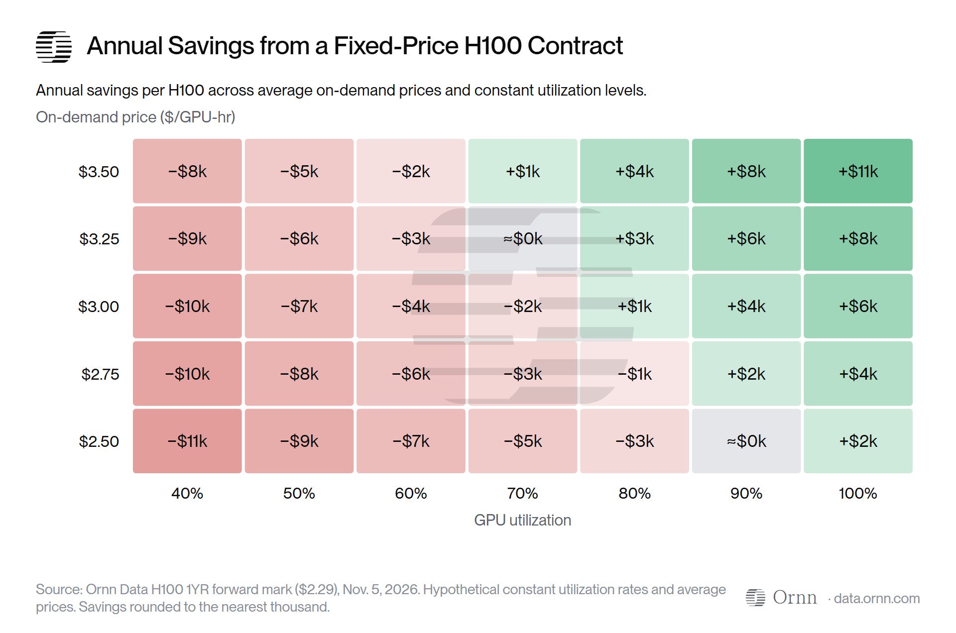
For a lab operating at 80% utilization, at an average on-demand price of $3.00/hour, the commitment would save approximately $1,000 annually per H100. But if the average spot price fell to $2.50/hour, that same commitment would instead cost the lab approximately $2,500 more than renting on demand.
At scale, with GPU fleet sizes ranging from smaller labs carrying single-digit GPU clusters to frontier labs with tens of thousands of GPUs, even modest changes in utilization can turn into millions of dollars saved or lost.
Breaking Even
In our heatmap, we showed examples of how utilization and on-demand prices can interact to determine the optimal value of a GPU commitment. It is important to note, however, that we assumed an average price throughout the year. In reality, price fluctuations can dynamically change the value of a commitment over time.
Let’s consider an AI lab hypothetically entering a one-year H100 reservation on November 5, 2025. On that date, an H100 rented on demand for $1.90/hour.
We do not have an observed one-year forward mark from November 2025, so we reconstruct a hypothetical rate using the 26.9% one-year discount observed in the one-year H100 term curve, as of November 5, 2026. Applying that discount to the historical on-demand price gives us a fixed contract rate of approximately $1.39/hour.
We then calculate the cumulative break-even utilization for each day of the following year, comparing the fixed $1.39 rate against the average on-demand price observed from the beginning of the contract through that date.
The resulting curve can be read as the percentage of reserved GPU capacity a buyer would have needed to consistently use, from the start of the contract up to each given date, for the commitment to have been cheaper than renting on demand.
Assume a lab maintains a constant 70% utilization throughout the year.
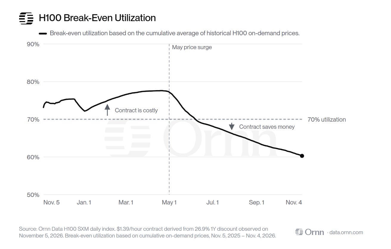
At the beginning of the period, the lab would have needed approximately 73% utilization to justify its commitment. At the lab’s 70% utilization, renting on demand would initially have been cheaper, and therefore preferential.
Over the next few months, H100 rental prices fell while the contract rate stayed fixed. By April 2026, the lab would have needed to average nearly 78% utilization since the start of the contract just to break even. Otherwise stated, it would have spent roughly 11% more under the contract than it would have renting by the hour over the same period.
Then, in May 2026, on-demand H100 prices rose sharply. The lab’s contract rate stayed at $1.39 per GPU-hour, while the average price it would have paid on demand since November began to climb. That brought the break-even utilization down.
By early June, the cumulative break-even threshold fell below 70%. The savings since the May price jump had more than offset the extra cost of the reservation in the first few months. For the first time, the lab was ahead on the contract, when compared against buying on-demand.
By the end of the year, the lab would have needed to use only about 60% of its reserved capacity to break even. At our assumed 70% utilization, it would have saved nearly $2,000 per H100 over the full year.
This is just one scenario in which we fix a hypothetical contract price and assume constant utilization, but it demonstrates how fluctuations in on-demand prices can change the economics of a take-or-pay commitment over its lifetime. Even if a buyer gets its utilization forecast exactly right, a rise in on-demand prices can turn the same reservation from a bad deal into a good one.
Not All Utilization Is The Same
So far, we’ve assumed that the lab uses exactly 70% of its reserved GPU capacity every day. This simplifies our calculations, but it overlooks another important source of uncertainty in the equation: when a lab uses their compute.
An inference provider might see demand rise during the day, fall overnight, and dip on weekends; an enterprise AI application might see demand rise during the workweek and fall over the weekend. A model developer might require substantial compute for intensive training runs, followed by periods of much lower demand.
All three could average 70% utilization annually, but the timing of their compute consumption could be very different.
To picture how these different workload schedules impact the economics of the contract, we ran a Monte Carlo simulation using three hypothetical workload schedules: steady inference, weekly cyclical demand, and intermittent model training.
Steady Inference: We simulated relatively consistent demand around 70% utilization, introducing small day-to-day fluctuations. That gives us a baseline for seeing how much the timing of GPU use matters in the other scenarios.
Intermittent Training: We simulated alternating periods of high and low demand, with training runs lasting 7-21 days at nearly full capacity (98%), followed by 5-16 days of much lower utilization (30%). These are your model developers (specifically neolabs), which might require substantial compute for intensive training runs before scaling back until the next one.
Weekly Cyclical: We simulated a recurring weekly pattern, with higher GPU usage during weekdays (85%) and lower usage over weekends (32.5%). These are your enterprise AI applications, whose compute requirements might rise and fall alongside their customers' working schedules.
For each workload, we generated 1,000 possible daily utilization schedules, each averaging exactly 70% across the year.
We then calculated what those schedules would have cost using the same historical H100 on-demand prices and compared the results against our hypothetical $1.39/hour reservation.
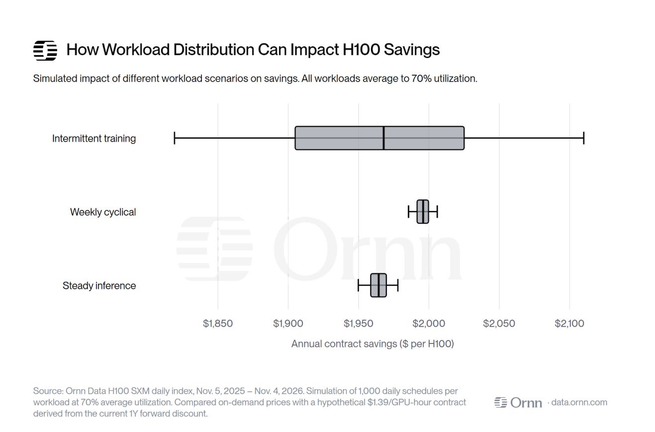
While all three workloads averaged the same 70% utilization, the variability in their savings differed considerably.
Steady inference produced the most consistent outcomes, as relatively stable daily demand meant that no single period had much influence on total costs. Weekly cyclical workloads showed similarly little variability, since their higher weekday demand and lower weekend usage followed a predictable pattern.
Intermittent training, however, produced a much wider range of outcomes. With compute demand concentrated in intensive training runs lasting several weeks, the timing of those runs mattered considerably more. A neolab whose training coincided with high on-demand prices would have saved more by locking in its rate, while one whose training occurred during cheaper periods would have benefited less.
For buyers, this means that two labs with different types of workloads expecting the same annual utilization may face very different levels of uncertainty about whether a long-term commitment will pay off.
The Importance of Secondary Markets
Now we find ourselves back at the buyer’s original problem. Buyers of compute—AI companies—want to grow, and their ambitions depend on them securing the optimal amount of their core input at the optimal price. However, they still need to calculate their utilization carefully, as overcommitting to capacity they may not use can quickly erase the savings from a discounted contract.
Secondary markets can be the wind in the sails of compute buyers, derisking ambitious utilization assumptions by providing the possibility of reselling excess capacity. Rather than leaving unused GPU capacity as a sunk cost, labs could recover some of their contractual commitments by selling capacity they no longer need.
In fact, this possibility changes the economics of committing to compute in the first place. By lowering the utilization required for a long-term reservation to break even, secondary markets could give labs greater confidence to secure capacity ahead of demand, making long-term contracts more attractive to buyers who might otherwise hesitate to commit. This is one reason we built Ornn Compute.
GPU prices in this article
The latest Ornn Compute Price Index (OCPI): executed on-demand rental prices, per GPU-hour.
More research
- Will Anthropic Grow Into Its Compute Bill?
What Anthropic’s $895 billion in compute commitments imply about its growth trajectory.
- Introduction to Compute Markets #1: The Primary Market
How computing capacity is sold directly to customers: reserved, on-demand and spot.
- The Compute Certainty Tax
How much revenue GPU clouds give up to make their fleets financeable.